Free space path loss is not useful in all link budgets

Most link budgets are based on Friis transmission formula [1]. However, they generally use a more contemporary expression [2] instead of the original one. Both these formulas are also discussed in [3] with a derivation based on radiometry.
Using the contemporary formula has many consequences as values like free space path loss (FSPL), transmit equivalent isotropic radiated power (EIRP), and receive gain G_r are included in the formula.
The received power is then given by:

$P_r = G_r \, P_t \, G_t \, \left(\frac{\lambda}{4 \pi d} \right)^2 = G_r \times EIRP \times FSPL$

The free space path loss is given by:

$FSPL=\left(\frac{\lambda}{4 \pi d}\right)^2$

The equivalent isotropic radiated power is the product of the transmitted RF power by the transmit antenna gain:

$EIRP=P_t \, G_t$

Use of the contemporary Friis formula

From this equation, it seems that you must know the frequency, the transmitted power and antenna gain, the receiver antenna gain, and the distance between the transmitter and the receiver to compute the link budget.
In other words, the system has already been designed and you have very little room for change and improvement.

This is a big problem if your work is to design the system and your first task is to determine the frequency, the distance, the antennas’ dimensions and the transmit power.
Using an Excel sheet and finding values by trial and error is time-consuming and does not guarantee you will get the best solution.
Working in this way is also a hindrance when an innovative solution is needed.
Except for computing the link budget as a function of distance on a designed system, the contemporary Friis transmission formula is useful only in the case where the mission of the system imposes the transmit and receive gains whatever the frequency and distance.

One example is the point-to-point transmission where you cannot impose or know the pointing direction of the antennas. In that case, your constraint is to use antennas with low directivity and gain, possibly omnidirectional antennas. You find the classical saying that a lower frequency and a smaller distance are better for the link budget.

Use of the original Friis formula

Not all system missions follow this path. If you can point both antennas precisely and the main constraint for both antennas is dimensions or areas, you had better use the original Friis formula [1]:

$\frac{P_r}{P_t}=\frac{A_r \, A_t}{d^2 \, \lambda^2}$

This formula uses neither the EIRP nor the FSPL. It shows that the highest possible frequencies (even better, optical frequencies) will give you the best link budget. This is the case for inter-satellite links which use Ka-Band or optics.

Both expressions are related by the value of the gain G of an antenna as a function of its effective area A_e and frequency or wavelength [2, 3]:

$G=\frac{4 \pi A_e}{\lambda^2}$

New proposed formula

Now if your constraint is to provide reception in a given coverage area such as a country or continent from some orbit, or part of a town from a telephony base station, you may use another formula that simply uses the ratio of receive antenna effective area to coverage area.

$\frac{P_r}{P_t}=\frac{A_r}{A_{coverage}}$

Figure 1: Reception by an antenna effective area in a coverage area

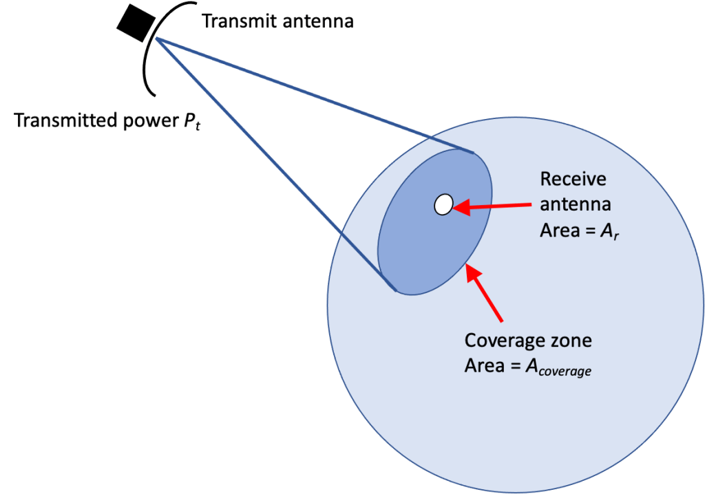
The coverage area A_coverage is measured on facets orthogonal to the transmit antenna’s direction. It is roughly equal to the area of the portion of sphere subtending the same solid angle as the geographic coverage and at an average distance from the transmitter or the product of the geographic area by the cosine of the angle between the area and the average transmitter direction. It is obtained more exactly by integrating the products of small solid angles by the square of the distance to the transmitter in all this geographic coverage.
Such a transmit antenna is called an isoflux antenna, it sends the same flux or power density per square meter in all useful directions.
The receive antenna effective area is also supposed to be orthogonal to the same direction.
This is only a first-order formula and you will have to design the isoflux transmit antenna to efficiently and homogeneously spread all the transmit power in the coverage area without any spill-over.
This formula shows that the link budget is independent (in the first order) of frequency and distance.
In addition, this formula does not need the values of the gains of bi-oth antennas nor the equation giving them for the link budget computation. It can be obtained by direct computation of the maximum power flux that can be obtained from a transmit power on a given area. It can be applied to shaped and over-dimensioned antennas with beam widths much larger than the diffraction limit. The formula is independent of how an antenna works and the diffraction theory.
Quite evidently, higher frequencies will have more atmospheric losses. Larger transmit antennas will be needed in cases of larger distances, lower frequencies, and smaller coverage areas. Transmit antennas will also be more complex if the coverage area is not a simple circle or ellipsis.
But antenna efficiency and atmospheric losses will also occur in a link budget based on EIRP and FSPL. In addition, you would have to consider antenna’s complexity and compute its gain even before having chosen the frequency and the distance (and angle of coverage).
For a classical parabolic antenna, the link budget worst case is obtained at the edge of coverage where the antenna gain is 3 dB less than the maximum gain. The effective area may be 50% to 70% of the physical area, giving another loss of 1.5 to 3 dB. More complex-shaped antennas may have less variation between maximum gain and minimum or edge of coverage gain but they have a lower ratio between effective and physical areas.
This last link budget formula is important because it shows that the same power per square kilometer (power flux) and the same receive antenna effective area are necessary for a given capacity transmitted either from a geostationary (GEO) satellite or from a low Earth orbit (LEO) constellation. This is quite contrary to what can be wrongly deduced by just looking at the free space path loss.
The LEO satellite antenna is smaller because the distance is smaller, but a larger number of antennas and satellites are necessary to transmit to the same coverage area.
The ground antenna to a GEO satellite is easier to make larger because it does not have to track the satellite in real time.

Conclusion

Depending on the system to be designed and the main constraints on both antennas (dimensions or gain) you must choose between 3 expressions of Friss transmission formula, two of which use neither FSPL nor EIRP.
To improve the link budget, one expression favors lower frequencies, the second one favors higher frequencies and the last one is independent of frequency giving completely different compromises for optimum systems.

Reference

[1] Friis, H.T., “A Note on a Simple Transmission Formula”, IRE Proc. 34 (5), May 1946, pp. 254–256.
doi:10.1109/JRPROC.1946.234568
[2] https://en.wikipedia.org/wiki/Friis_transmission_equation
[3] Shaw, J. A., “Radiometry and the Friis transmission equation”, American Journal of Physics. 81, 2013, pp. 33–37.
doi:10.1119/1.4755780

Jacques Sombrin